Computational Geometry

Key Resources

Textbook: Computational Geometry - Algorithms and Applications
Coursera Course: For the Problemset and Implementations (Till Part 5)
Philipp Kindermann’s Lectures Series (Part 6 and Onwards)
Various Random Resources found on the internet!
- Geom Algorithms
- CP Algorithms

Overview

To learn computational geometry, these are the steps/resources I used,

Week 1 - Week 5: Coursera - Computational Geometry
- For theory, read from book and/or random resources off the internet. Philipp’s lectures are also available for this.
- Focus on the problemset for the course.
- Recommended Prerequisite: Good understanding and practice of DSA. Some of the problems have tons of edge cases!
Week 6 - Week 10: Philipp Kindermann’s Lecture Series
- This part is more theory oriented and covers Voronoi Diagrams, Delaunay Triangulations too.
- Again some parts can be followed up from the book as well.
- Recommended Prerequisite: Basic graph theory (maximal planar graph, duals), basic DSA (analyzing time complexity)

General Implementation Aspects

Use slope pairs
Triangle orientation check (sign of area)
Sum of area of triangles to form interior
Ray out of a point inside intersects polygon odd times
Check line segment intersections by checking orientation of each of the four points (not two!)
It also helps to plot sample testcases for debugging
Modulo to cyclicly iterate through points of a Polygon
Carefully inspect, input/output format as well as edge cases

// My Header - (Used mostly STL instead of OOP)
#define ll long long
#define x first
#define y second
typedef pair<ll,ll> vertex;
typedef pair<ll,ll> point;
typedef pair<double, double> ppoint;
const ppoint INF_POINT = {2e9, 2e9};
const double EPS = 1e-16;

Week 1

1. Point and Vector (Triangle Sign Check)

This will be used in most future problems as well. The most generalized template is below. Note that area is actually twice the actual area.

int trisign(ppoint a, ppoint b, ppoint pt){
    double area = a.x * b.y + b.x * pt.y + pt.x * a.y - a.y * b.x - b.y * pt.x - pt.y * a.x;
    if(area > EPS){
        return 1;
    }else if(area < -EPS){
        return -1;
    }
    return 0;
}

2. Point in Triangle

Principle is the sum of the 3 individual triangles (2 vertices, 1 point) would be equal to total area (3 vertices).

3. Point in Polygon

Take ray from point to infinity
Check intersection with each line segment O(N)
Parity of the number of intersection determine inside(odd) or outside(even)
Ignore if line segment coincides with the ray.

This is used again in future problems like 4-1/4-2. Draw a ray from P to INF_POINT. Check the if the no. of intersections are odd or even. Make sure an endpoint is not counted twice - that’s why semi-open interval is checked (semi_check_intersect).

bool inbetween(ppoint a, ppoint midd, ppoint b){
    double minx = min(a.x, b.x);
    double miny = min(a.y, b.y);
    double maxx = max(a.x, b.x);
    double maxy = max(a.y, b.y);
    return (minx <= midd.x && midd.x <= maxx) && (miny <= midd.y && midd.y <= maxy);
}

// Only check semi-interval [s1, s2) intersection [d1, d2]
bool semi_check_intersect(ppoint d1, ppoint d2, ppoint s1, ppoint s2){
    int s1_side = trisign(d1, d2, s1);
    int s2_side = trisign(d1, d2, s2);
    int d1_side = trisign(s1, s2, d1);
    int d2_side = trisign(s1, s2, d2);
    if(s1_side*s2_side == 0 && d1_side*d2_side <= 0){
        // If segment lies completely inside we can ignore it; So check if strictly only s1 is present
        return (inbetween(d1, s1, d2) && !inbetween(d1, s2, d2));
    }else if(s1_side*s2_side <= 0 && d1_side * d2_side <= 0){
        return 1;
    }
    return 0;
}

bool point_in_polygon(vector<vertex>& poly, pair<double, double> p){
    int ray_intersects = 0;
    int n = (int)poly.size();
    for(int k = 0; k < n; ++k){
        ray_intersects += semi_check_intersect(p, INF_POINT, poly[k], poly[(k+1) % n]);
    }
    if(ray_intersects % 2 == 0){
        return 0;
    }else{
        return 1;
    }
}

4. Points in Convex Polygon

The steps I used were as follows -

Get Centroid: Choose 3 non-colinear points (trisign)
Sort by Angle: Array of pairs slope_pairs which stores {atan2(points[i].y - centroid.y, points[i].x - centroid.x), i} and then sort.
Binary Search by Angle (Helper Function): pair<ll, ll> binsearch_angle(vector<pair<double,ll>>& angle_pair, double angle_val) gives the pair of indices of the two vertices.
Check in triangle: Use the previous part to check if point in the triangle given by binsearch_angle

Week 2

Convex Hull Algorithms
- Graham Scan
  1. Initialize a pair of points in S
  2. Add new point
  3. Check if orientation of (n-2)nd point with ((n-3)rd, nth) point is left(ccw)/right(cw) (and 0)
  4. Else pop the 2nd last point
- Andrew’s (Preferred - NlogN for sort)
  1. Take line (leftmost or minx) point & (rightmost or maxx) point
  2. Sort Points in x-coords
  3. Partition all other points (by orientation) into Lower or Upper according to below/above the partition line. (stable or resort)
  4. Run Graham Scan and pop 2nd last element if right(for Upper Partition) or left(for Lower Partition)
Points to Note: - Andrew’s Scan can also be thought similar to a sweep line - At every event point(p) check orientation of last point in S(n) wrt to S(n-1) and p - Convex Hull can also be used for other polygons (see Unit Circle’s questions)
- Jarvis March
  1. Take lowest point in H
  2. Take 2nd point with smallest polar angle in H
  3. Take last (n-1) and (n-2) points as line
  4. Find smallest polar angle point wrt. this line
  5. Repeat till 1st point is found

1. Convex Polygon Check

Check if polygon is convex. Stable Partition points to upper part and lower part (like Modified Graham’s). Check (convex_check) if all Up points have no lefts. Check again if all Down points have no rights.

bool convex_check(vector<pair<ll,ll>>& points, int invsign){
    ll sz = points.size();
    for(int i = 0; i < sz-2; ++i){
        // NO Left(>0) if Down, NO Right(<0) if Up
        if(trisign(points[i], points[i+2], points[i+1]) == invsign){
            return 0;
        }
    }
    return 1;
}

invsign is an integer which is 1 or -1, depending on lower or upper hull.

2. Convex Hull

Convex hull follows similar to the convex hull check.
For each vertex, we check while(hull_size + 1 >= 3)
If trisign(hull[hull_size - 2], points[i], hull[hull_size -1]) matches our invsign then pop the 2nd last vertex, Or else break out of the while loop to check the next vertex.
Function Header: void construct_convex_hull(vector<pair<ll,ll>>& points, vector<pair<ll,ll>>& hull, int invsign);
After construct_convex_hull for both partitions, we zip the upper and lower Hulls. Thus forming the CCW convex hull.

3. Tangents to Polygon

See geomalgorithms.com for excellent explaination of technique. As stated, we need sign(left point) != sign(right point) for tangent In our case to find left and right tangents, we can put a condition like this, inside our loop iterating through each point.

int signl = trisign(left_pt, points[i], pt);
int signr = trisign(points[i], right_pt, pt);
if(signl != signr){
    // CCW => pt lies L/R wrt. leftpt
    if(signl == sign || signr == -sign){
        return points[i];
    }
}

where sign is given by whether we want left or right tangent.

4. Union of Convex Hulls

Take any point Z inside Convex Polygon A. If Z is also inside B, sort the points by angle and apply graham scan. If Z is not inside B, remove inner chain and apply Graham’s Scan on outer chain. OR Just apply Graham’s Scan to all the points since both algorithms have worst case, NlogN. This may however be slightly less optimal. (But it works :-))

Week 3

1. 2 Line Segment Intersections

See CP Algorithms for technique. Helper functions for this include, trisign, inbetween, determinant are used. Remember to check for ‘No Common Points’ for both determinant = 0 and not. Watch out for corner cases. (Tons of them!)

2. Polygon Intersection

Either Clipping (Sutherland Hodgman) or Line Sweep (Shamos-Hoey) could be used. For clipping, see G4G. The Algorithms are as follows,

Sutherland-Hodgman
- First choose a polygon
- Cut out 2nd polygon from first (check orientation at each line and split half-plane)
- Go through the vertices of the 2nd polygon and check if next vertices crosses the line or not. ~O(NM) time
- Also, for convex + non-convex
Shamos-Hoey (Sweep-Line Like) - (N + M) vertical lines from vertices - Obtain inner fragment at each line (inner up and inner down) - 4 lists of vertices (upper, lower) - Only for convex + convex
```
Within the same TC but slightly less optimal, a simpler approach using all the previous functions can be used.
```
Simply, find all line segment intersections and check point in polygon for each vertex. Then just order points cw / ccw by sorting by angle from centroid. See D3 Mike’s ObservableHQ for an awesome visualization.

3. Intersection of Horizontal and Vertical Segments

This is briefly discussed in ‘Competitive Programming Handbook by Antti’. Scan the the edges and classify and store as horizontal/vertical segments. Store in start, tuples of the form

{x1, 2, vptr} for vertical segments
{xmin, 1, hptr} and {xmax, 3, hptr} for horizontal segments The operations are 1(Add eventpt), 2(Intersect with vertical), 3(Remove Endpoint). Sort the start array, and perform a line sweep over it. Use order-statistic tree (policy-based ds) for the status. (or implement similar RBT using nodes)

// Horizontal Segment (height)
vector<ll> hzlevel;
// Vertical Segment (height, range)
vector<pair<ll,ll>> vlevel;
// Starting Point Tuples (xcoord, operation, index)
vector<vector<ll>> start;

// In operation 2 we check intersects like this,
lo = status.order_of_key(vlevel[ix].first);
hi = status.order_of_key(vlevel[ix].second+1);
intersects += hi - lo;

4. Intersection of Set of Segments

Classic Sweep Line for Segment Intersections
- Consists (key vars)
  - Event Point
    - Upper (or left) Endpoint of Segment is p (U(p))
    - Lower Endpoint of Segment is p (L(p))
    - Intersection/Internal Point of segment is p (C(p))
  - (Q) Event Queue of found event points
  - (S) Set of of all Segements (Array)
  - (T) Set of Status (RB Tree?)
  - Event Queue set to check if already present?
- FindIntersection(S)
  - Initialize Q and T
  - Push first U( p ) endpoint (and corresponding line segment/index) in Q
  - While Q non-empty, HandleEventPoint
- HandleEventPoint(p)
  - Consists of U, L, C
  - Generate L( p ) and C( p ) from adjacent segments in T
  - Segments of $L(p) \cup U(p) \cup C(p) \geq 2$
    - Report intersection p
  - Delete L( p ) since segment ends
  - Delete C( p ) to swap (2nd priority to U)
  - Insert U( p )
  - Insert Back C( p ) (finish swap)
  - If there is no U( p ) and no C( p )
    - FindEventPoints(sl, sr, p) where sl, sr are the adjacent segments of p in T
  - Else
    - Take leftmost segment of U( p ) union C( p ), ie (topmost priority) as sl
    - Take left neighbour of sl in T, s1
    - FindEventPoints(sl, s1, p) // top Segments intersections
    - Take rightmost segment of $U(p) \cap C(p)$, ie (least priority) as sr
    - Take right neighbour of sr in T, s2
    - FindEventPoints(sr, s2, p) // bottom Segments intersections
Key Features for any Sweep Line
- Event Point (often coordinate-compressed)
- Status Set containing elements important for current event point
- Line sweeps across some direction (Obvious!)

Unfortunately, I wasn’t able to code this one up. However, geom algorithms explains with code the approach to doing this.

Week 4

1. Diagonals of any Simple Polygon

For diagonals, one technique is to first check if diagonal intersects with any other polygon line segment. Then check if Point-in-Polygon for the midpoint, to know if it is inside/outside. So, trisign, inbetween, semi_check_intersect, check_intersect and point_in_polygon are needed. Note that check_intersect includes endpoints unlike semi_check_intersect.

intersect diagonal_check(vector<vertex>& poly, ll i, ll j){
    int n = (int)poly.size();

    // Check Intersections
    for(int k = 0; k < n; ++k){
        if(k == i || k == j || (k+1) % n == i || (k+1) % n == j) continue;
        int res = check_intersect(poly[i], poly[j], poly[k], poly[(k+1)%n]);
        if(res == 1) return crossing;
    }

    // Check if Midpoint in polygon. Assumption: diagonal does not intersect
    pair<double, double> midd = {(poly[i].x + poly[j].x)/2.0, (poly[i].y + poly[j].y)/2.0};
    if(point_in_polygon(poly, midd)){
        return inner;
    }else{
        return outer;
    }
}

2. Ear-Cutting Algorithm for Triangulation of Convex Polygons

Steps -

Preprocess: If for every vertex, adjacent vertices form inner diagonal. Mark as Ear. ~O($N^2$ for diagonal_check)
Start processing ears in-order from a starting vertex (Try to maintain order in which they are checked)
Delete Current Ear Vertex from the polygon (& is_ear) vector. Insert (diagonal with adjacent verts and the pt) as a triangle.
Check if vleft, vright is a ear (~O(N))
Stop when ear-list is empty or polygon has less than 3 vertices (all vertices are done!)

Time: $O(N^3)$ (Sum of $N^2$ operations)

After preprocessing the ears in the is_ear array, the algorithm proceeds as follows,

// Set start point
int st = 0;
while(n > 3){
    // Start loop at previous triangle endpoint
    for(int j = st; j < st + n; ++j){
        int i = j % n;
        if(is_ear[i]){
            // Find First Ear and Delete
            vector<vertex> res_triangle = { poly[(i - 1 + n) % n], poly[i], poly[(i + 1) % n] };
            triangles.pb(res_triangle);
            is_ear.erase(is_ear.begin() + i);
            poly.erase(poly.begin() + i);

            // Update Polygon and check ears
            n = (int)poly.size();
            // Lower Vertex
            is_ear[(i-1 + n) % n] = check_ear(poly, (i-1 + n) % n);
            // Upper Vertex (new index -> i % n)
            is_ear[i % n] = check_ear(poly, i % n);

            // Set start of next iteration
            st = i;
            break;
        }
    }
}

Finally, add remaining polygon into triangles. The check_ear functions checks diagonal_check(from 4-1) on the neighbouring vertices. It also helps to plot testcases like this,

3. Monotone Polygon Triangulation

Triangulation of strictly y-monotone polygons. See MCS481 Slides for a pretty good psuedocode or the Book is also great. For Diagonal check part, time complexity would be high therefore it is better to use Concavity Check with trisign instead. Remember to add diagonals from last (lowermost) vertex also. sidemap is used to store Left/Right and vertex is the merged sorted vertex list.

void triangulate_monotone(vector<point>& verts, map<point, bool> sidemap, vector<polygon>& diags){
    int sz = (int)verts.size();
    deque<point> rack = {verts[0], verts[1]};

    for(int j = 2; j < sz-1; ++j){
        point vlast = rack.back();
        // Process Vertex
        if(sidemap[verts[j]] != sidemap[rack.back()]){
            // Opposite Sides
            while((int)rack.size() > 1){
                diags.pb(vector<point>{rack.back(), verts[j]});
                rack.pop_back();
            }
            rack.pop_back();
            rack.push_back(vlast);
        }else{
            // Same Side
            rack.pop_back();
            // rack.back() should be inward wrt. vlast and verts[j] -> i.e, match sign of side of vlast
            while(rack.size() && check_concave(vlast, rack.back(), verts[j], sidemap[verts[j]])){
                diags.pb({verts[j], rack.back()});
                vlast = rack.back();
                rack.pop_back();
            }
            rack.push_back(vlast);
        }
        rack.push_back(verts[j]);
    }
    // Add diags from all verts in stack (except top and bottom) to lowermost vertex
    rack.pop_front();
    rack.pop_back();
    for(auto v: rack){
        diags.push_back(vector<point>{verts[sz-1], v});
    }
}

4. Number of Triangulations of a Convex Polygon

From the wikipedia page, A convex polygon with n + 2 sides can be triangulated to n triangles by non-crossing lines.
Number of different ways of triangulation is Catalan Nos.
For any triangulation, there would be exactly 2 vertices that don’t need to be joined by a diagonal.(or whose degrees stay the same!) So, catalan nos. is on the $n-2$ vertices connected by diagonals.
The $\sum c_i c_{n-i}$ Form: Recurrence relation is the breaking of the polygons by one of the diagonals.

Week 5

k-D Trees
- Base Structure: BST
- Stores values like BST, but instead of ordering only by value like BST, it needs to order by k params.
- This is done by selecting a splitting criteria, like for 2D: alternate between ‘X’ and ‘Y’ parameters based on whether the depth is even/odd.
2D Layered Range Trees
- Base Structure: Red-Black Tree or balanced BST
- See differences between some well-known trees.
- 2D Layered Range tree stores points in its associated array, and optimized for “which points fall within a given interval” queries.
- The assoc array of point v is the two-pointer zip (merge-sort) of 2v and 2v+1 vertices.
- It can be represented similar to 2D segment tree, but value contains “the points themselves”. (segtree consists of sum of no. of points)
- Both 2D layering range tree and segment trees can be used interchangeably.
- Fractional Cascading is technique to store binary_searched index of the element as pointer. So $O(logN)$ extra factor isn’t needed. Each element of assoc array of point v also contains pointers to 2v and 2v+1 nodes arrays’ binary_searched(lower_bound) index.
2D Priority Search Tree
- Base Structure: Binary Heap or Priority Queue (Scaled up to 2D).
- Shows one-sided unbounded range of values.

1. Closest Point

Simple binary-search implementation as points have only 1 parameter.

2. Number of Points in Rectangle

The easiest implementation in via a Cartesian Tree. (similar to Kdtree) My code is a 2D Segment Tree however I recommend using an OOP approach with Cartesian Tree instead!

This is was approximate workflow while designing 2D Segment Tree. See CP Algorithms’s compression of 2D segment tree for ideas. Fractional Cascading for speeding up!

Below are the design notes for the code.

General Design -
  - buildx, buildy, queryx, queryy
  - Range compression (See cp-algorithms.com tips)
  - NlogN memory and (logN)^2 time per query
Construction -
  - Vector with all x-coords sorted
  - Vector with all y-coords sorted for each node of segtree[x] to lowerbound/upperbound y indices
  - Within each node of segtree[x], store `segtree[][y]` with compressed size 4*log(Sumx_r - Sumx_l)
Query -
  - Search equivalent indices for x-coords in vec
  - Get each node from segtree query
  - Search equivalent indices for y-coords in each vvec[v_x]
  - Get each node sumval from segtree[v_x] query
Variable Names-
  - v -> root vertex
  - l, r -> current left/right segment of coords
  - L, R -> required left/right segment
  - Lyc, Ryc -> c indicates coordinate and not index
Current Progress -
  - Correct Answer and correct Memory Limit
  - Time Limit Exceeded in Building Segtree
      - Building Time: ~ 4min 45 seconds
      - Query Time(for 30000 queries): ~ 5min (9 min 45s in total)
Optimization -
  - Get rid of binary search for both x & y and instead check coord value
  - Remove coord compression but keep construct_order_y
  - Make D&C of segment tree run on array with unique elements (order_x, order_y) instead
  - Fractional Cascading:
      - Store relation(starts) between unique array (order_x) and points
      - So, construct_order_y does not require to binary search index (remove extra logN factor)

The Segment Tree is built on the unique x-coordiniates (order_x) array and 2nd dimension in unique y-coordinates (order_y). It assumes that points do not repeat!

CTags-like Overview of global variables,

const ll SZX = 30001;
const ll INF = 1.5e9;

// Segment Tree : 4*SZX and 4*SZY (still only NlogN memory since dynamic length arrays!)
vector<ll> segtree[4*SZX];

// Unique x-coordinates of points
vector<ll> order_x;

// Unique Y-coordinates of (vx)th segment tree (4*SZX and SZY)
vector<ll> order_y[4*SZX];

// List of all points in sorted x-coordinate order
vector<pair<ll, ll>> points;

// Fractional-Cascading like map of unique x indices of order_x to non-unique coordinates' indices in points
ll starts[SZX];

Overview of Functions,

// Query the (vx)th segment tree
ll queryy(ll vx, ll vy, ll ly, ll ry, ll Lyc, ll Ryc);

// Build (vx)th segment tree on the basis of y-coords (USES queryy for 2*vx, 2*vx+1 segment tree values)
void buildy(ll vx, ll lx, ll rx, ll vy, ll ly, ll ry);

// Construct the base array for the (vx)th segment tree (Called within buildx)
size_t construct_order_y(ll vx, ll lx, ll rx);

// Builds the segment tree and proceeds to call construct_order_y and buildy
void buildx(ll vx, ll lx, ll rx);

// Query the x-coordinate and proceed to call queryy
ll queryx(ll vx, ll lx, ll rx, ll Lxc, ll Rxc, ll Lyc, ll Ryc);

The start array is constructed in preprocessing stage before buildx. construct_order_y uses start array for copying y-coords of original array (so no logN factor from lower_bound).

Building: buildx -> construct_order_y -> buildy -> (either fill value 1 or queryy)

Query: Format input to lower/upper endpoints -> queryx -> queryy At both queryx and queryy(similar but with lxy rxy), ll lxc = order_x[lx], rxc = order_x[rx]; line is used. The lxc rxc (coordinates of query points) are used for all comparisons except for calculation of midpoint where lx rx (positions) are used.

3. Closest Pair of Points

K-D Tree Implementation. See Rosetta Code or Stanford ACM’s Notebook. For intuition on K-D Trees see Josh Hug’s lectures General Parameters that can be tuned,

Distance Metric
- Euclidean Metric
- Chessboard Metric (Used for this problem)
- Manhattan Metric
Splitting Criteria (X or Y based)
- Parity of Depth/Height of current node
- Larger of Width or Height of bounding box of current node

Week 6 - Point Location and Trapezoid Maps

Lec 1 - “Where the hell am I?”

Planar Subdivision: A set of polygons that form a large polygon.(Like a map of states of a country)
Partition into vertical lines or slabs at every vertex (like Shamos Hoey)
Naive Implementation
- Query: Traverse two binary search trees - find vertical lines (bound on x), find region (bound on y);
- Space Complexity can be n^2 if two full BST

Lec 2 - Decreasing Space Complexity

Refinement: The Partition of Planar Subdivision S into Slabs induced by vertices. These Partitions would be trapezoids (or degenerate ones).
Trapezoidal Map: Splits the trapezoids of a refinement. Very useful technique for space partitioning or mapping regions in general.
Unlike the previous partition by vertical lines, this partition only has lines that end at another edge or outer rectangle.
Side: Segment of max length contained in boundary of face of trapezoid
Trapezoidal partition with $n$ segments have, $T(S) \leq 2n + 2*2n + 4$(segment endpoints, vertical lines, boundary rectangle) vertices and trapezois $\leq 3n + 1$
Constructing Trapezoid - Find each up, down left, right endpoints for each trapezoid. Time: 3N + 1 = O(N)

Below is an image of a trapezoidal map of ’line segments’ from this GAS, the same can be done for polygons as well.

Lec 3 - Randomized-Incremental Algorithm:

O(NlogN) expected preprocess time
O(logN) query time (not worst case optimal but randomized)
Expected Query Time by Backward Analysis (See Lec04 of series)

Lec 4 - Data Structure Trapezoid Cartesian DAG

Trapezoidal Map Data Structure For 2D: Cartesian D.A.G.
Make sure to split Trapezoid on map (so it isn’t n^2 time)
Unlike Tree, Cartesian DAG will just have pointer to that trapezoid

Lec 5 - Query Time for Trapezoid Cartesian DAG

LogN Query time (Amortized)
Backward Analysis (summation 1/i)
Size: O(N + 13N) = O(N) (13N comes from $\sum(3i + 1)*(4/i)$)
Construction: NlogN

Week 7 - Voronoi Diagrams & Post Office Problem

Lec 1 - Post Office Problem

Post Office Problem: Which is the closest Post Office to place P?
Answer: Voronoi Diagram with Euclidean Distance Metric. (Map of region closest to that point)

Lec 2 - Definitions in Voronoi Diagrams

Voronoi Cell: $$ V(p) = { x \in R^2: d(x, p) < d(x, q) \forall q \in P\ - {p}} $$
For Voronoi Cell, Think of definition of Ball in Topology but using relative distances instead of a constant epsilon
Voronoi Edge: $$ V(p) = { x \in R^2: d(x, p) == d(x, q) \forall q \in P\ - {p}} $$

Lec 3 - Overall Shape of Voronoi Diagrams

Lemma: Vor( P ) consists of atmost (2n - 5) vertices and (3n - 6) edges
Proof of Lemma from Euler’s Polyhedra Formula (Dual is Delaunay Triangulation and Maximal Planar Graph => 3n - 6)
For infinite voronoi diagrams, set dummy vertex at infinity
NOTE: Voronoi Vertices != Voronoi Cells (or Faces or Sites)
Voronoi Vertex: Circle at vertex ‘x’ has atleast 3 points on it’s largest (circumcircle which does not contain a site/face) $$|C_p(x) \cap P| \geq 3$$
Voronoi Edge: For edge P to P’, there is a vertex ‘x’ which has P and P’ on it’s largest (circumcircle which does not contain a site/face) $$\exists x \in E(P, P’) st.,\ \ |C_p(x) \cap P| = {P, P’}$$

Lec 4 - Computing Voronoi Diagram

BF: Line Segment Intersection, Half Plane Intersections > $O(N^2)$ time
Naive Line Sweep: Event Points are not known before swept
Fortune’s Algorithm or Optimized Line Sweep:
- Parabolas at the visited vertices form the equidistant line
- Directrix is the Line Sweep at point P, and focus is the visited vertices
- Beachline($\beta$): The lowerbound of each of the parabolas (from the visited vertices so far) merged together.
- The intersection points of the parabolas as the line is swept form the edges of the voronoi diagram.
- See this for demo. Also, this post for explaination.
Beachline Event Points
- Site(Face) Event: New Sitepoint is found => New Arc is created
- Circle Event: Sweep Line reaches lowest point of circle containing 3 Site Points => Arc of the inner site point is deleted. Voronoi Points are the centre of the circle formed.

Lec 5 - Fortune’s Line Sweep Algorithm

See PVigier’s Blog for implementation resources.
Also see this post by Jacques
Key Functions
- Find New Circle Event Points (Site Event Points are already known)
- Handle Circle Event (once processed; calls findNewCircleEvent)
- Handle Site Event (once processed; calls findNewCircleEvent)

Week 8 - Delaunay Triangulations

Lec 1 - Height Interpolation

Triangulation: Planar subdivision with all inner faces triangles and outer face is Convex Hull
Since Maximal Planar Graph => (3n - 6) edges. But outer face is CH and needs triangulation (3 - h) edges => 3n - 3 + h edges in total

Lec 2 - Angle-Optimal Triangulation

Height Interpolation Optimization by choosing a better triangulation
Angle-Optimal Triangulation to avoid skinny triangles (this causes disparity in length Vs width - based height interpolations)
Angle vector $A(T)$ of Triangulation $T$ is the angles of all triangles in sorted order
A Triangulation is more optimum if Angle vector is lexicographically better than the other. i.e., $A(T_{optimal}) > A(T)$
The best triangulations are called Angle-Optimal.

Lec 3 - Edge-Flips & Legal Triangulations

Edge e is illegal in Triangulation T if triangulation obtained by flipping edge e, T’ has $A(T’) > A(T)$
Use Extended Thales Thm (Thales++), i.e., check angles by taking circumcircle around edge e
Angle-Optimal is always legal.
A triangle is legal iff it has no illegal edge

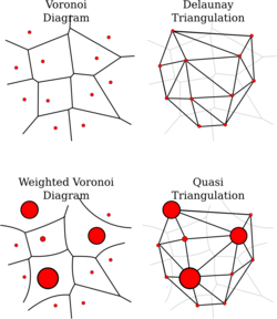
Lec 4 - Voronoi Diagram & Delaunay Triangulation

Delaunay Triangulation: Straight Line Drawing of the Dual Graph of Voronoi Diagram
Proof
- Take circumcircle on any point in edge between sites p-q in Vor(P)
- Consider another edge u-v and show crosses lead to contradiction
Alt Definition: Delauanay Triangulation iff $\forall \Delta \in T : int(C(\Delta) \cap P) = \phi$
AKA: Empty Circumcircle property of D.T.

Lec 5 - Correctness and Computation

A triangulation is legal iff it is Delaunay
Proof
- Back Relation: By Empty Circumcircle Property and Thales++, D.T. is legal
- Forward Relation:
  - By Contradiction, Take a triangle p-q-r and circumcircle. where T is legal
  - Take point s in circumcircle. Now, we need to maximize angle of chord at s. (p-s-q)
  - Take neighbouring triangle p-q-t, t lies outside circumcircle.
  - Get contradiction: angle q-s-t > angle p-s-q (but this is maximal)
If pointset P is general position(i.e. No 4 points lie on an empty circle) then D.T. is unique and angle-optimal.
If pointset P is not general position, then all D.T. have same minimum angle but may not be angle-optimal.
D.T. can be constructed in $O(NlogN)$
Angle-Optimal Triangulation in non-general position P, can be constructed in $O(N^2)$ time. Holes (4+ points on empty circle) can be filled by trying out each flip.

Below is an image also showing weighted voronoi diagrams and their corresponding delaunay triangulations,

Week 9 - Convex Hull in 3D

Lec 1 - Complexity and Visibility of CH

(Upper Bound Theorem) General Time Complexity of Convex Hull in d dimensions: $O(N^{\lfloor d/2 \rfloor})$
In 3D, Surface of the Polyhedra forms a Planar Dual Graph => atmost (3n-6) edges and hence linear complexity. Similar for higher dimensions.
Construction by Random-Incremental Algorithm
Visibility:
- If we project rays from point P to Convex Polytope.
- The project rays that are 3D Tangent to the polytope form a ring/shadow, the point that form this is called Horizon.(Last visible edges)
- Region facing towards P bounded by Horizon is the Visible region.
Define Conflict Graph and create bipartite relation of points with facets. And mark out which facets are visible.

Lec 2 - Randomized Incremental Algorithm

Pseudocode/Approach of adding vertex to CH3
TC: $O(N^2)$ (Randomized from $O(N^3)$; not worst case optimal)

Lec 3- Analysis

Expected No. of Facets Created by CH are bounded to atmost (6n - 20)
Degree bounded by 6 for the vertices other than initial 4-point CH3, so 6*(n-4) + 4
See this Tutorial on 3D CH for simple implementation as well as some optimized version.
Can be further optimized with Configuration Spaces
Higher Degree CH are worst case optimal accordingly with Upper Bound Thm.

Lec 4- Convex Hull & Half-Plane Intersections

Assume a mapping/relation from spaces P1 and P2, where (‘primal is the dual of the dual!’)
- Line in P1 -> point in P2 (P1 is Dual of P2)
- Line in P2 -> line in P1 (P2 is Dual of P1)
Convex Hull of a point set in P1 => Set of Lines in P2
- Traversing the lines corresponding to Lower Hull of P1 alongside intersections, give the Upper Envelope. Similarly for Upper CH.
- Incidence Preserving: Every point in P1 gives Line in P2. So CH region gives area bounded by upper and lower envelope.
- Order Preserving: Maintains an ordering through the mapping.
Scaling to 3D: CH3 of points gives 3D Wrapping/Envelope of 3D Lines

Lec 5- Voronoi Diagrams Revisited

Distance to Unit Parabola (From Projection of point q to tangent at p’) = intercepts $(pq)^2$
Take: A (set of planes/halfplanes) have an Upper Envelope (or Supremum or Least Upper Bound 3D Parabola). The planes are thus 3D Tangents to the 3D Parabola or Envelope.
When this is projected to the plane,
- Voronoi Centres/Faces/Sites = (Intersection points of Planes and 3D Parabola)
- Voronoi Edges = (Line Segments that for the Intersection of Planes)
- Voronoi Vertices = (Intersection of 3 or more Planes)
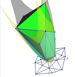
Take: 3D Convex Hull of (Intersection of Planes and 3D Parabola). The 3D Parabola is now the Lower Envelope (or Infimum or Greatest Lower Bound) of the (3D Convex Hull).
When this projected to the plane,
- Delaunay Vertices = (Intersection of Planes and 3D Parabola) or (Points of 3D Convex Hull)
- Delaunay Edges = (Edges of 3D Convex Hull)
See Video for Demo

Below image is from DesignMentor, showing delaunay triangulation as a projection of a 3D Convex Hull

Week 10 - Motion Planning

Lec 1 - Point Shaped Robots

Trapezoidal Map for Path with Obstacles. Finding Path: O(NlogN) Construction and O(N) query

Lec 2 - Configuration Space

Degrees of Freedom: 2D(2 translation x, y + 1 rotation \theta) = 3, 3D(3 translation x,y,z + 2 rotation $\theta, \phi$) = 5
Configuration Polygon: Polygon s.t. foreach point in ConfPol, Robot at point (x, y) (R(x, y)) intersects with obstacle polygon(Pi). (If point robot, then this is just the obstacle polygons.)

$$ CPi = {(x, y): R(x, y) \cap P{i}} $$

Lec 3 - Characterizing Configuration Spaces

Minkowski’s Sum (For Polygon!): $S_1+S_2={p + q : \forall p \in P, q \in Q}$ where p, q are point vectors
Geometric Representation: Replace Copy of S1 in every point of S2 to form the new shape. (or Vice versa; commutative)
Inversion in Polygon Algebra: Rotate polygon by 180 around origin. $S2 =-S1={-p : \forall p \in P}$
Configuration Polygon: $CP = P + (- R(0, 0))$ (where ‘+’ is minkowski sum)

Lec 4 - Complexity and Computation

Atmost n+m edges in minkowski sum(S) of P (n edges) and Q (m edges)
We can define a map of each edge of S to a pair (i, j) of the edges in P, Q.
Quadratic Algorithm: Convex Hull of points where at each corner of P, Try every rotation of Q
Linear Algorithm: (Two-Pointers-like) Choose Bottom-Right most point for both. And move p_ptr or q_ptr based on which has a smaller angle.

Lec 5 - Pseudodisks

Def: Pair of Planar Objects (P1, P2) form a pseudodisk if (bound-> boundary, int->interior),
- $bound(O1) \cap int(O2)$ is connected
- $bound(O2) \cap int(O1)$ is connected
Consider 2 convex polygons with disjoint interiors.
- Let d1 -> direcion where P1 more extreme, similarly d2.
- Then P1 is more extreme in [d1, d2] or [d2, d1]. Or in a circle, one boundary part has P1 more extreme and other with P2.
For P1, P2, take CP1 = P1 + R, CP2 = P2 + R. Then proof by contradiction. So (CP1, CP2) have to be pseudodisks.

Lec 6 - Union Complexity

For Convex Polygons P, Q, R,.., the total union has atmost 2*(n+m+l+..) vertices. (since every (two or less) crossings can be mapped to a vertex)
For constant complexity convex robot R, translating among S disjoint objects with N edges. We can preprocess in $O(N (logN)^2)$ and compute collision-free path in O(N)
Approach
- Triangulate Polygons if Not-Convex to make it convex (NlogN)
- Compute ConfPol for each Obstacle Polygon (N)
- Compute Union of Obstacles by sweep line (N $(logN)^2$)
- Mark out Trapezoidal Maps etc.
- Query: Find path in complement of unionConfPol with help of Trapezoidal Map