Introduction
In this post, we delve into the mental model (or abstract feeling) of things being continuous Vs discrete. In the direction of continuous vs discrete ideas, we look into signal processing, numerical methods and random ideas.
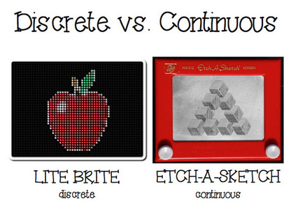
Poster originally by mathbytori.blogspot.com
Throughout this post, the terms ‘discrete’ and ‘continuous’ are somewhat loosely defined.
A simple intuition on continuous and discrete would give us,
| Discrete | Continuous |
|---|---|
| Distinct, seperate and countable | Fluid, mostly singular |
| Dotted Line | Normal straight Line |
| Scattered | Unionized |
| Set of Integers $Z$: Distinct points on the number line | Set of Real Numbers $\Re$: Continuous line on the number line |
| Sets not dense (in any metric space) | Set is dense (in any metric space) |
| Non-seperable Metric Space(like discrete metric space) | Seperable Metric Space |
| Discrete Probability Distribution | Continuous Probability Distributions |
| Histograms | Kernel Density Estimates |
| Digital Image Processing | Analog Image Processing |
| Discrete Delaunay Triangulations | Continuous Voronoi Diagrams |
| Discrete Time Signals | Continuous Time Signals |
| Sum of many discrete rectangles | Area under a continuous curve |
| Discrete Factorials | Continuous Gamma Function |
| Discrete Transforms | Continuous Transforms |
| Discrete Recurrence Relations | Continuous Differential Equations |
A common trend to notice is that discrete things tend to take a finite or countable set of values.
Discrete Signals Vs Continuous Signals
Moving to more concrete definitions, Let us take the example of Continuous vs Discrete in the context of Signals. This divides us into four parts shown below,
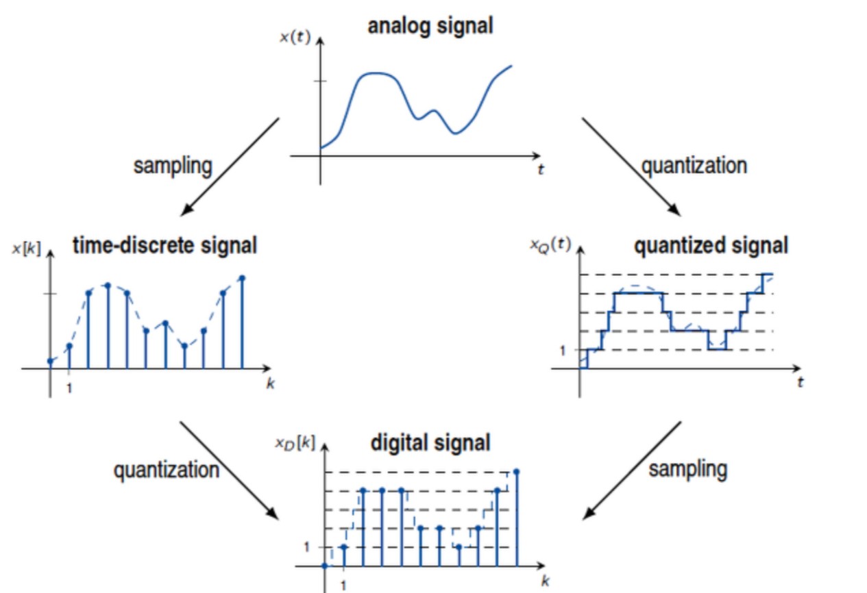
Clockwise: CT Analog, CT Digital, DT Digital, DT Analog
The differentiating factors are,
- Discrete time (DT) Vs Continuous time (CT)
- Analog signal Vs Digital signal
Here, digital signal and analog signals are both continuous in time but the CT digital signal has only a discrete set of values for the ouput $y(t)$.
In this post, the ideas of ‘digital’ and ‘discrete’ may be mixed because ‘digital’ signals are still discrete in the y-axis.
Area under a Continuous Curve Vs Sum of many Discrete Rectangles
Considering the area under the curve for any continuous function $y(t)$, the area is given by $\int_{t_0}^{t_n} y(t)$
However, if we consider the digital equivalent of this function (by quantizing the input), the area under the curve can just be the sum of distinct rectangles.
So we get, $\int_{t_0}^{t_n} y(t) = \sum_{i=0}^{n-1} y(t_i)$.

Wikipedia: Riemann Sum (taking midpoints)
Taking the value at each midpoints and summing the rectangles we get, $$\int \limits_a^b m(x)dx = \lim_{n \rightarrow \infty} \frac{|b - a|}{n} \sum_{k = 1}^{n} m(a + k \frac{|b - a|}{2n})$$ So, as we make the partition intervals smaller ($\lim_{n \rightarrow \infty} \frac{1}{n}$), this sum becomes closer to the actual integral.
A mid-riser or mid-tread quantizer in signal processing, would be analogous to a Riemann sum except for one point. The quantizer divides the signal $y(t)$ into discrete bins (and reconstructs). However, the riemann sum would divide the input $t$ into discrete bins.
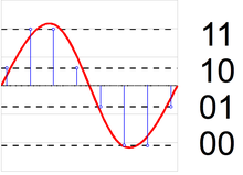
Wikipedia: Quantization of Signal with 4 Levels
Instead of partitioning the continuous function into rectangles, we could take the function values at two points and break it into trapezoids. (Trapezoidal Rule)

Wikipedia: Trapezoidal Rule
Similarly, we can approximate with even more function points to get the other Newton Cotes Formulas.
So, all these summations functions are approximations to integrations (each with a same or faster convergence).
Discrete Factorials Vs Continuous Gamma Function
Considering another seqn of numbers, $$1, 1, 2, 6, 24, 120, 720 …$$ Can you guess the sequence?
For any given sequence in $N$, there will always be infinitely many continuous functions in $\Re$, that satisfy the sequence.
But one special function that represents this is the gamma function, $$ \Gamma(z) = \int_0^{\infty} x^{z-1} e^{-x}dx$$
Here, $$ \Gamma (n + 1) = n!$$ thus captures the factorial function.
(Note that however the gamma function is continuous only in $\Re^{+}$.)
For many sequences which are a discrete recurrence relation, a continuous generating function can be also found.
Discrete Vs Continuous - Fourier-Like Transforms
Another interesting and useful concept when dealing with signal processing, is the fourier transforms. It is a very essential way to transfer a random signal (think square, triangular, wavy, crazy or any time-based oscillation) into a mixture of sine ways of different frequencies. 3blue1brown has an amazing visual introduction to the fourier transform.
When considering fourier transforms, there are numerous generalization for different signals. The types of transform depends on the 4 differentiating factors,
- Discrete Signal or Continuous Signal
- Periodic Signal or Aperiodic (Infinite Period) Signal
- Transform or Inverse Transform (Analysis or Synthesis)
- Imaginary exponent Vs Complex(re + im) exponent in equation
Considering the normal transform in real domain, varying points 1 and 2, we get the following table,
Fourier Series Vs Fourier Transform
Similar to the CTFT and DTFT, there is also inverse CTFT and inverse DTFT. This article has a nice table,

Medium: Fourier Transform Table
‘Complex Fourier Series’ is the same as ‘Continuous Time Fourier Series’
Switching the last parameter 4 from purely imaginary to complex exponents, give us two new transforms -
- Laplace Transform (Continuous Domain)
- Z - Transform (Discrete Domain)
In the transforms, the real component gives us the $e^x$ curves and the complex exponent gives us the $e^{ix} = cos(x) + isin(x)$ curves.
An ugly inconsistency
Considering the laplace transform to be, $$ X(s) = \int_{-\infty}^{\infty} x(t) e^{-st} dt $$ An intuitive definition of Z-transform would be, $$ X(z) = \sum_{-\infty}^{\infty} x[n] e^{-zn} $$ where z just like s would be defined by $z = \sigma + i\omega$
Unfortunately, due to ease of usage in digital signal processing the definition of z-transform was made rather unintuitive. Hence, it is given by, $$X(z) = \sum_{-\infty}^{\infty} x[n] z^{n} $$ where $z = e^{sT}$ (instead of $z=sT$)
From this we see the mapping,
$j\omega$ axis for the Laplace transform $=$ unit circle for the Z transform
See this thread to know more. Another stackexchange thread, also points out why the laplace transform cannot be defined the other way around.
Discrete Recurrence Relations Vs Continuous Differential Equations
Consider two alien species in two different planets with no natural predators and sufficient resources to grow.
- The first alien species breeds naturally with its growth twice its current population (population growth rate 200%).
- The second alien species reproduces using binary fission. So, one alien essentially splits into two new alien creatures. And all the alien species undergoes this binary fission every new years’ eve.
Both these cases could be modelled as,
- $y’ = 2y$ where $y$ is the population, and $y’$ is it’s derivative (the population growth rate).
- $a_n = 2 a_{n-1}$ where $a_n$ is the population in year $n$
Notice that in case of alien species no. 1 we are modelling it as a continuous differential equation whereas in the case of alien species no. 2 we are modelling it as a discrete recurrence relation.
In case of alien species no. 1, we have to solve the differential equation which gives us, $$y = a_0 e^{2t}$$ where $a_0$ is a constant representing the original population of aliens.
So if there where 1 million aliens, originally, there would $e^2 \approx 7.34$ million aliens after just one year.
For alien species no. 2, it is relatively straightforward to see that a population of 1 million aliens would be 2 million after the first year.
It is also intuitive to notice that after any $n$ years the solution to this is, $$ a_n = a_0 2^n $$
This similarity between the population growth equations can be seen better by modelling the recurrence relation as an diferential equation.
Consider the population after 3 years, it is 4 times the population after year 1 so,
$$a_3 = 2 * ( 2 * a_1 )$$ $$a_3 - a_1 = (2^2 - 1) a_1$$
So from this we could say for any general points a_{n+k} and a_n,
$$ \Delta y \approx \Delta a_n = a_{n + k} - a_n = (2^k - 1) * a_n $$ $$ \Delta t \approx \Delta n = (n + k) - n = k $$
$$ \lim_{\Delta n \rightarrow 0} \frac{\Delta a_n}{\Delta n} = \lim_{\Delta k \rightarrow 0 } \frac{(2^k - 1) * a_n}{k}$$
Taking derivative on both numerator and denominator with the El ‘Hospital’ rule,
$$ \lim_{\Delta n \rightarrow 0} \frac{\Delta a_n}{ \Delta n} = ln(2) a_n $$
Modelling $a_n$ as $y$ and $n$ as $t$ we have,
$$ y’ = ln(2) y $$ $$ y = a_0 e^{ln(2) t} = a_0 2^t $$
Or better expressed as,
$$ a_n = a_0 2^n $$
Another way to look at the two alien species is that,
- The 1st alien species is a 100% compound interest which is continuous compounded.
- The 2nd alien species is a 100% compound interest which is compounded annually.
Note that instead if we take any other coeffecient too this would work!
For 2nd Order and above
It also works similarly for second order differential equations and second order recurrence relations. The technique to solve 2nd order ODE and 2nd order RR are the same,
- Put the solution as $y = C_0 e^{rt}$ or $a_n = \alpha^n = e^{ln(\alpha)n}$
- Solve the quadratic equation or “characteristic equation” that transpires to get the general solution
- Find the particular solution, this could be with the help of specific boundary conditions etc. and combine.
Without getting into too much detail, For the general solution of 2nd order ODE with distinct roots, $$ y = C_1 e^{r_1 t} + C_2 e^{r_2 t}$$ and for repeated root, $$ y = C_1 e^{r_1 t} + C_2 t e^{r_2 t}$$
For the general solution of a 2nd order recurrence relation with distinct roots, $$ y = C_1 r_1^n + C_2 r_2^n = C_1 e^{ln(r_1) n} + C_2 e^{ln(r_2) n}$$ and for repeated root, $$ y = C_1 r_1^n + C_2 n r_2^n = C_1 e^{ln(r_1) n} + C_2 n e^{ln(r_2) n}$$
Other Interesting References
- Can’t find a generating function for factorials
- A philosophical and cognitive science view of analog, digital, continuous and discrete.
- Baby Steps of Statistics
- Fourier Transforms 101
- For mental models in other domains, refer Farnam Street Blog or Super Thinking Book
- Try to find an anology for discrete vs continuous, with separable and non-separable spaces. Good Resources: Separable Spaces, Discrete-like non-separable subspaces in separable spaces, Database of Topological Counterexamples