Principles of Economics

Introduction

These are my notes for POE. The notes were written using markdown and vim (see iamcco/markdown.nvim plugin) and Pandoc (with eisvogel template). Feel free to collaborate to the Online Version of POE Notes. These are only supplementary notes and NOT Lecture Notes. Some useful resources.

• ACDC ECON Tutorials by Jacob Cliffords for both Micro and Macro
• Khan Academy - Microeconomics

Elasticity Curves Part

Elasticity : % change quantity / % change price $$\epsilon = \frac{ \% \Delta Q}{\% \Delta P}$$

(Similar to sensitivity)

• Inelastic

  • monopoly
  • necessity
  • small E = Not much choice
  • E < 1 ( or slope > 45)
  • TR decreases for increase in quantity

• Elastic

  • perfectly competetive
  • large E = plenty choice
  • E > 1 ( or slope < 45)
  • TR increases for increase in quantity

Types of Elasticity

• Cross Price Elasticity sensitivity of A has, $\epsilon_{cross\ price} = \frac{ \% \Delta Q\ of\ B}{ \% \Delta P\ of\ A}$
• Income Elasticity $\epsilon_{income} = \frac{ \% \Delta Q}{ \% \Delta Income}$

Other Terms

• Consumer Surplus = Buyer’s Max - Price (Upper Triangle)
• Producer Surplus = Price - Seller’s Min (Lower Triangle/Part)

  See CH-13 Monopoly and Antitrust for Graph and Explaination

6 - Household behavior and Customer Choice

• Household Demand Factors- Price, Income, relative prices preferences
• Budget Constraint (Eqn)

1. Utility

   • Rule of Diminishing Marginal Utility, Saturating curve of TU
   • Utility Maximizing Rule $\frac{MU}{Price}$
   • Diamond-Water Paradox Water becomes granted so diminishing MU and downward-sloping (double derivative +ve)

2. Income and Substitution Effect

   • Income effect is the change in consumption of a product due to the relative change in price of product (well-being) Parallel Shift of Budget Constraint
   • Substitution effect is the relatively cheap as compared to competitors hence shift in purchasing towards that product (not substitutes) Angle turn along the Indifference Curve

   1. Income Effect on Labour Supply Curve Labour Supply Curve is Backward Sloping Curve

      • Substitution is upward slope part

      you have to work hard coz you earn more now

      • Income Effect is reverse slope part
        

      if you become rich, then you wanna party and do play!

3. Indifference Curves

   • Curve that yields same total utility

   consumer is indifferent between any points on curve

   • Diminishing MRS (law of diminishing utility)

   that’s why it slopes asymptoetically

   • Chooses highest curve touching budget constraint

   slope of indifference curve = slope of budget line

7 - Production Process: behavior of Profit-Maximizing Firms

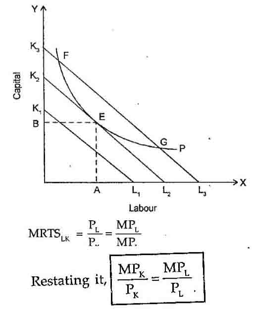
Analagous to Chapter 6 but slightly different. Production process is in terms of inputs and outputs. K(capital)-L(labour) is the new Price-Quantity with MRTS slope

1. Behavior of Profit Maximizing Firms

   • how much output to supply
   • how to produce that output
   • how much of each input demand

   1. Profit and Economic Costs

      • Total Revenue, Total Cost, Economic Profit
      • Most Important factor of production for opportunity cost = capital
      • Rate of return : annual net income % of total income (breaks into shares?) so it’s just enough to keep owners happy (like risk-free bonds)
      • Normal Rate of Return = zero profit equilibrium point
      • Input Type
        • Fixed
        • Variable

   2. Short Run and Long Run

      • short run : fixed rate of production (no scaling up/down or no exiting/entering)
      • long run : firms can choose to expand or contract

   3. Others-

      See Optimal method of production chart in CH-8 below

2. Production Process

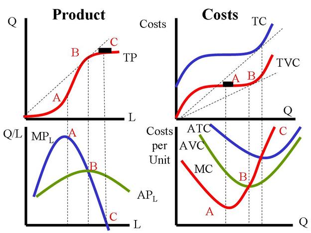
   Total, Average and Normal Product of Labour. See Curves in CH-8

   • Equivalent-Law of diminishing returns (MP of Labour)

   • 3 Stages of TP, AP, MP Curve-

     1. MP reaches maximum (double derivative 0)
     2. AP = MP
     3. MP = 0 and thus TP is maximum

3. Equivalent behavior (Others)

   Producer Market	Consumer Market
   Isoquant	Indifference Curve
   Isocost	Budget Constraint
   X	Labour(L)
   Y	Capital
   MRTS	MRS
   Cost-Min Eq	Utility-Max Eq

8 - Short Run Costs and Output Decisions

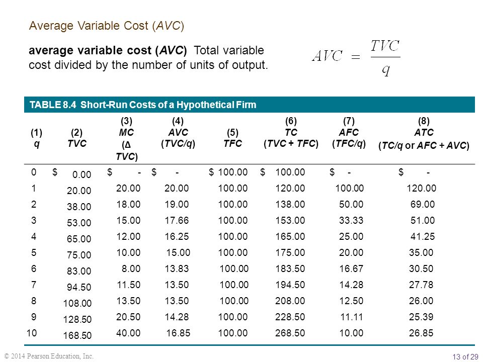
TC (overhead), TFC, TVC, AFC, AVC, MC (=MVC), AP, MP See Curves.

1. Types of Costs

   Main Types Costs

   • Fixed Cost
   • Variable Cost

   Analyze costs as

   • Total Cost
   • Average Cost = $\frac{TC}{Q}$ where Q is quantity at that time
   • Marginal Cost = increase in TC for production of 1 more unit output

2. Cost Curves

   • Variable costs depends on -
     • techniques of production
     • prices of inputs required
   • Plot has x-axis = Output and y-axis = type of cost

   1. Fixed Cost Curves

      Spreading Overhead

      • Fall of total fixed cost by increasing quantity (small cost per quantity; down asymptoete)
      • TFC still remains line parallel x-axis(Output)

   2. Variable Cost Curve

      Increases with quantity

   3. Marginal Cost Curve

      slight decrease till max then increase all the way

      • Marginal Cost increases with output (since no change in scale of production
      • diminshing returns = increasing marginal cost

   4. Notes on Curves

      • Marginal Costs is slope of TVC
      • The dip point (minima) of MC is the inflection point of TVC
      • MC cuts AVC at min of AVC and ATC at min of ATC
      • Short Run Curves

   Where MC crosses is where others stop falling

   

3. Output Decisions and Summary

   • Marginal Revenue Curve and Demand Curve identical in a perfectly competetive market
   • Profit Maximizing- Take $MR = MC$ (where Price from Demand Curve cuts MC for competetive)
   • Firms will produce only as long as MR > MC
   • Profit Maximizing Rule is the Loss Minimizing Rule

4. Types of Questions-

   • Table-based question (fill the table of TFC, TVC, AVC, MC….)
   • Equation of TC in Q given
   • Sketch graphs for different situations

9 - Long Run Costs and Output Decisions

• Terms
  • Shutdown Point TR < TFC (or P < AVC)
  • Long term contraction if TR < TC (Contracts and then exits)
  • Operating Profit: TR - TVC (may be losses!)
  • Economic Profit Vs Accounting Profit at 0-profit point

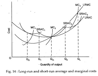
Long Run Average Cost Curve

The graph is split into 3 parts-

1. Economies of Scale (Beginning Drop) : More Cost but More Quantity = Less ATC
2. Constant Returns (Constant Line at Min) : Same as short run
3. Diseconomies of Scale (Upward after Dip) : More Cost but not much more Quantity = More ATC

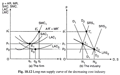
Long Run Industry supply Curve

Decreasing Cost Industry Above

LRIS Calculation

• Demands expands to D2
• Prices Rise to P1'
• New Firms enter and supply shifts to SRS3
• Price goes down to P3
• Based on decrease in price (Decreasing cost) or increase (Increasing Cost)
• Since P3 < P0 so LRAC decreases and Decreasing Cost-Ind

10 - Labour and Land Markets

• Shifts in Input Demand Curves
  • Demand for Outputs
  • Quanitity of Complementary and Substitute
  • Price of other inputs
  • Technology Change
• Profit Maximizing

Labour Market

• Derived Demand: Indirect demand like Labour not Goods and Services
• Marginal Product of Labour: Additional Output produced by adding another unit of labour
• Marginal Product of Labour Increases then decreases. e.g-

  Too many cooks, spoil the broth….. too few cooks, can’t make the broth?

• Marginal Revenue Product MRP(L): Price of output X MR(L)
• Market Labour Supply Curve
• Profit-Maximizing (from MR = MC): MRP(L) = Wage(W)
• In perfectly competetive firms, combine all MRP(L) have common price of output (see questions)

Land Market

• Demand Determinant: Price determined exclusively by its demand. Supply is Fixed (perfectly inelastic). e.g - Land
• Pure Rent: Return to factor of production with fixed supply

11 - Capital Market and Investment Decisions

Market Structures (and 15.1)

• Perfect Competition (E = $\infty$)
• Monopolistic Competition (Not Monopoly-Like!)
• Oligopoly
• Monopoly (E = 0)

15.1 Monopolistic Competition - Industry Characterstics

• Large no. of firm
• No barriers to entry
• Product Differentiation

13 - Monopoly and Antitrust

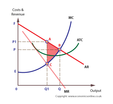
• Marginal Revenue -

  • For Monopoly, TR is max when MR = 0
  • For Competetive Firm, MR = price (varied by market)
  • MR has slope less (more -ve) coz Additional Output => Lower Price for more demand.

• Pricing and Ineffeciencies-

  • Firm produces Q at $MR = MC$ (at Q1) but prices Demand Curve (P1)
  • Leads to Dead Weight Loss (Allocated Ineffeciency) - unecessarily less customers = A-B-C Triangle
  • Consumer Surplus - Lost high pricing for rich customers = Triangle P1-A-F
  • Producer Surplus - Price of good higher than cost-to-manufacture = Area of E-C-P1-A

• Barriers to Entry -

  • Economies of Scale - Very Large (or high advertisement costs) (Predatory Pricing …See Oligopoly)
  • Patents - (Mostly Medicine Companies)
  • Government Rules - Laws favouring Gov Monopolies or through Lobbying
  • Ownership of Exclusive Capital - Own Diamond Mines etc.
  • Network Externalities - Dependant on the popularity of the product

• Social Costs of Monopoly -

  • Deadweight Loss (Depriving Customers of the product)
  • Rent-Seeking behavior (through lobbying and building Barriers)

14 - Oligopoly

• Measures for Oligopoly

  • HHI = Sum of Squared-Market-Shares (>1,800 for High)
  • CR (Conc. Ratio) = % Share of top n companies (>80% for High)

• Types of Oligopoly

  • Non-Collusive
    • Cournot’s Duopoly
  • Collusive (Can be Tacit or Non-Tacit)
    • Price Leadership
    • Cartels and Collusion

• Price Leadership - Dominant Firm decides market price for smaller firm.

• Predatory Pricing - Temporarily selling at artificially low price to kill competitors

• Cartel Duopoly - Use like monopoly with $MR = MC_1 = MC_2$

Cournot’s Model

• Assumptions- Identical Firms with homogenous products
• Response Func = Func of output of a Firm
• Inverse Demand Func - price of product
• Same Equilibrium for both firms
• Steps to solve
  • Equate $MR = MC$ for each firm
  • Output of each firm as func of other firm (Response Func)
  • Intersection of Responses (Can be plotted) is the Nash Eq.

Game Theory

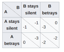
• Dominant Strategy - Player has a strategy which is better irrespective of the other’s solution
• Nash Equilibrium - All players play their best strategy (Need not be dominant-dominant!)
• Maximin Strategy - Low risk to maximize the min gain (opposed to minmax)
• Tit-for-tat Strategy - Response Based Strategy

• Prisoner’s Dilemma (see above) - Dominant-Dominant is not Nash Eq. (or best strategies)

20 - Intro to Macro

• Aggregate: To refer to sums only
• Recession/Slump or Expansion/Boom
• Depression = Long lasting depression
• Business Cycle: One cycle of slight recession and expansion
• Macroeconomic Concerns
  • Output Growth: Aggregate Output
  • Unemployment: unemployment rate not too low(business will not have labour) and not too high (jobless people)
  • Inflation and Deflation: Mild Inflation rate is required - Hyperinflation: rapid and devaluation (Venzuala, Turkey..) - Deflation: Nobody buys anything = No businesses (Japan)
• Circular Flow Diagram between Household, Gov, Firms, World

Class Notes Terms

1. Goods and Services Market
2. Financial Markets - Trading Securities (equities
3. Money Markets

Policies,

1. Fiscal Policy - Tax & Spending policies of Gov
2. Monetary Policies -
   • CRR: Cash Reserve Ratio (~4%)
   • SLR: Statutory Liquidity Ratio (~19.4%)
   • Repo Rate: Repurchase Agreement
   • Reverse Repo Rate: Reverse Repurchase Agreement

21 - Measure Outputs and Income (National)

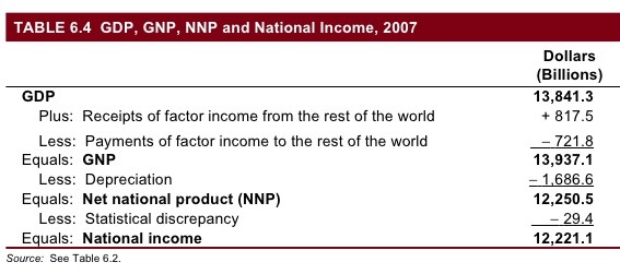
• Domestic Vs National : Region-based Vs Nationality(citizenship) based. See Honda Plant in Nagpur Example
• Gross Vs Net: Without Depreciation Vs True with Depreciation

• Note that depreciation is mostly considered only for net domestic-private investments and not others

Exclusions to GDP

• Final Goods and Services only not intermediate
• Value added method for calculating GDP
• Exclude Used Goods - No new production or revenue generation (except rent)
• Exclude Paper Transactions (like stocks and bonds but not broker fees) - No new production and only exchanges.
• Only domestically owned production - Only region based and not on citizenship (see GNP).

Expenditure Approach

$$GDP = C + I + G +(Ex -Im)$$

• Personal Consumption C: Household spending on goods and services

  • Durable: Furniture, cars…(longer lasting)
  • Nondurable: Food, clothing, gasoline..(short lived)
  • Services: Doctors, Educations…

• Gross Private Domestic Investment I: Purchase of new capital like

  • Residential: Houses etc.
  • Non-Residential: Machines, Tools, Plants
  • Change in Business Inventory: Goods produced for later sale in inventories

• Government Consumption and Gross Investment G: Goods (schools, government programmes, institutions…) and services (military salaries…)

  • Central (or Federal)
  • State

• Net Exports (Ex - Im):

  • Exports by the country shows production
  • Imports is production from other countries

Income Approach

This approach to GDP is from National income which is in decreasing order of magnitude from,

1. Compensation of Employees
2. Proprietors’ Income (Uncorporated businesses’ income)
3. Rental Income
4. Corporate Profits
5. Net Interest (!only interest from businesses)
6. Indirect Taxes minus subsidies
7. Net Business Transfers Payments by Businesses
8. Surplus from Government Institutions (often -ve unlike others)

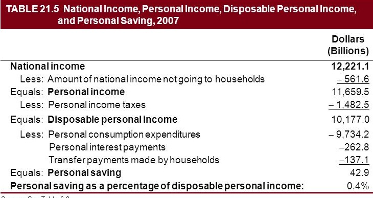
National Income to Personal Saving

Nominal Vs Real GDP

• Real GDP = Nominal GDP adjusted for price change
• Real Vs Nominal Output
• Fixed-Weight Procedure: Prices in base year as weights for reference
• GDP Deflator Method - Using series of % changes to measure overall price
• Problems of fixed-weight procedure

Limitations

• GDP does not reflect crime rate, increase in leisure time, pollution, domestic work and social ill.
• Informal Economy - illegal transactions and tax evasion
• Gross National Income per Capita as measure

25(.1, .2) - Money and Banks

Khan Academy - Money and Banking

Money as,

1. Medium of Exchanges (Not like barter, where we trade goods like cocoa)
2. Store of value - Asset that can be used to transport purchasing power (you can save for now and still spend later)
3. Unit of account (compare price of pizza and banana)

• Commodity Monies - Using cigerretes / Ramen as money in Jails.

• Fiat Money / Token Money - Money that is intrinsically useless (paper of rupee notes aren’t useful)

• Legal tender - What RBI says can be accepted as ‘money’ (ONLY currency!) see 51% torn part of dollar bill is legal tender in US

• Currency Debasement - Hyperinflation of currency value due to too much supply of currency (zimbabwe, post-war Germany, Venzuala…)

• Measuring Money Supply? Money Supply = Currency + Deposits

• Types of Money

  • M1 = Currency + Demand Deposits + Other Deposits
  • M2 = M1 + Saving Deposits with Post Office
  • M3 = M1 + Time Deposits with Bank ( Most Useful )
  • M4 = M3 + Total Deposits with Post Office Saving Organization (excluding NSC)

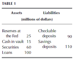
Creation of Money by Banks

(See Table 25.3 of Textbook for better understanding)